Introduction

우리 세상은 많은 modality가 존재한다. 그리고 관념적으로도 여러 modal의 네트워크들을 fusion시키면 uni-modal보다 성능이 더 좋게 나온다. 그렇다면 우리는 이러한 궁금증이 생긴다.

_multi-modal learning이 uni-modal learning보다 좋은 성능을 제공할까?_

저자는 이 궁금증에서 연구를 시작했고, 다음 두 가지를 중점적으로 살펴봤다.

• (When) 어떤 상황에서 multi-modal이 uni-modal 보다 성능이 좋은가?
• (Why) 무엇이 이런 성능을 유도했는가?

그리고 연구를 통해서 저자가 한 comtribution은 다음과 같다.

• Multi-modal learning을 population risk로 설명하고, 이는 latent representation quality의 bound 되어있다는 것을 밝혔다.
• 전체 modality의 subset으로 훈련시킨 network의 quality의 upper bound를 유도했다.
• Modality의 subset으로 학습시키면 성능이 하락한다는 것을 이론적으로 분석했다.

참고로 결론은 다음과 같다.

• Multiple modality는 그 modal의 subset보다 적은 population risk를 갖는다.
• 이는 multi-modal이 더 정확한 latent space representation을 학습할 수 있다는 것이다.

이제 하나씩 살펴보자.

The Multi-modal Learning Formulation

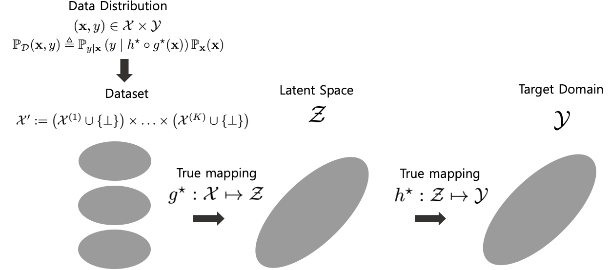
먼저 수식을 정리하자. K개의 modalities에 대해서 data는 \(\mathbb{x}:=(x^{(1)},\cdots,x^{(K)})\) 으로 표현한다. 이 때 \(x^{(k)} \in \mathcal{X}^{(k)}\) 이다. 우리는 K개의 modalities를 보유하기 때문에 전체 input data space는

\[\mathcal{X}=\mathcal{X}^{1} \times \cdots \times \mathcal{X}^{k}\]

로 표현된다. 그리고 target domain을 \(\mathcal{Y}\) , multi-modal의 공통된 latent space를 \(\mathcal{Z}\) 라 하자. 우리는 이제 true mapping을 다음과 같이 쓸 수 있다.

\[g^\star: \mathcal{X} \mapsto \mathcal{Z}, g^\star \in \mathcal{G}\] \[h^\star: \mathcal{Z} \mapsto \mathcal{Y}, h^\star \in \mathcal{H}\]

그렇다면 이제 우리는 \(\mathbb{x}\) 의 data distribution을 정의할 수 있다.

\[\mathbb{P}_\mathcal{D}(\mathbb{x},y)\triangleq\mathbb{P}_{y|x}(y|h^\star\circ g^\star(\mathbb{x}))\mathbb{P}_\mathbb{x}(\mathbb{x})\]

참고로 \(h^\star\circ g^\star(\mathbb{x})=h^\star(g^\star(\mathbb{x}))\) 로 합성함수를 의미한다.

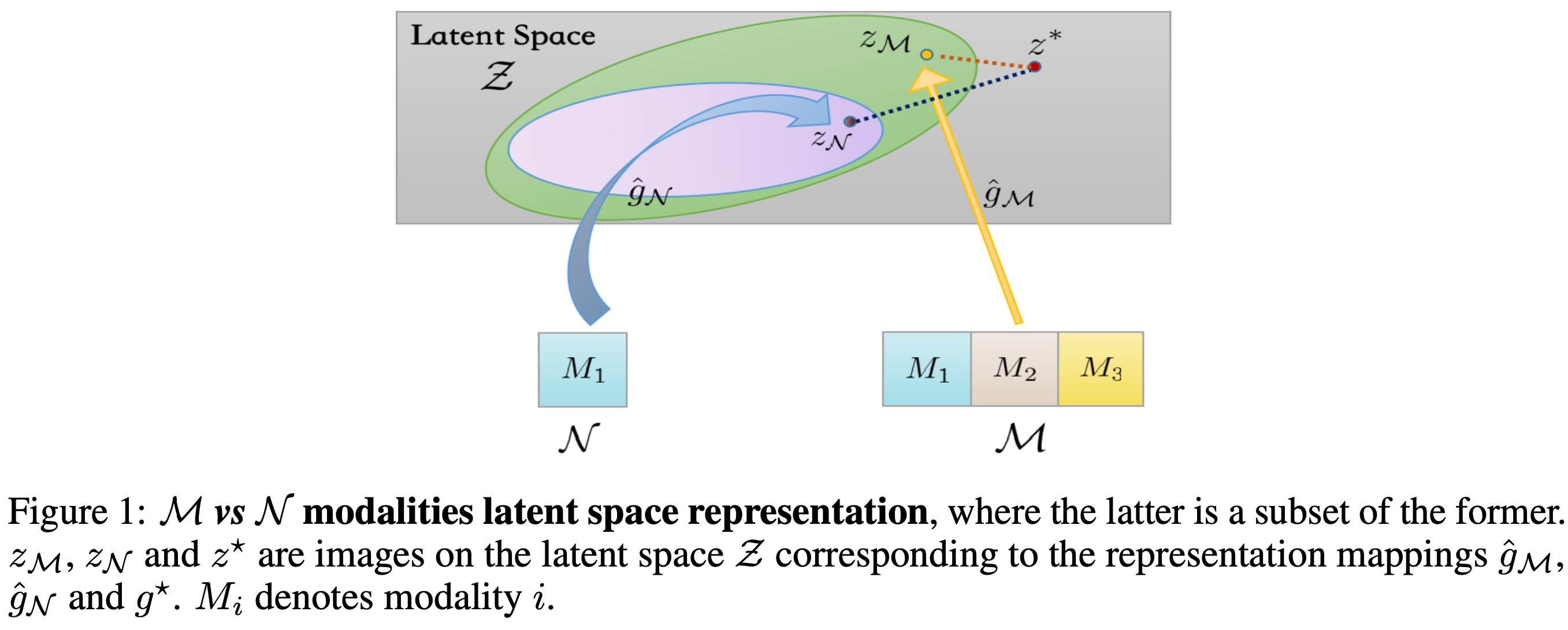
우리는 일반화를 위해 \(\mathcal{N} \leq \mathcal{M}\) 인 modalitie의 subset에 대해서 살펴볼 것이다. Modality의 superset을 정의하자.

\[\mathcal{X}^\prime := (\mathcal{X}^{(1)}\cup\bot)\times\cdots\times(\mathcal{X}^{(K)}\cup\bot)\]

이때, \(\bot\) 은 k번째의 modality는 쓰지 않는다는 것이다. 간단하게 시각화하면 다음과 같다.

이제 modalities를 선택하는 함수를 정의하자.

\[p_\mathcal{M}(\mathbb{x})^{(k)}= \begin{cases} \mathbb{x}^{(k)} \text{ if } k\in\mathcal{M} \\ \bot \text{ else } \end{cases}\]

이때, 우리는 다음과 같은 식을 만들수도 있다. \(p^\prime_\mathcal{M} := \mathcal{X}^\prime\mapsto\mathcal{X}^\prime\) 우리의 목표는 Empirical Risk Minimization (ERM) principle에 따라서 learning objective를 minimize하는 것이다.

\[\text{min } \hat{r}(h\circ g_\mathcal{M} \triangleq\frac{1}{m}\sum_{i=1}^ml(h\circ g_\mathcal{M}(\mathbb{x}_i),y_i) \text{ s.t. } h \in \mathcal{H}, g_\mathcal{M} \in \mathcal{G}\]

여기서 \(l\) 은 loss fuction이고, 최종적으로 정의하는 population risk는 다음과 같다.

\[r(h\circ g_\mathcal{M})=\mathbb{E}_{(\mathbb{x}_i, y_i)\sim\mathcal{D}}[\hat{r}(h\circ g_\mathcal{M})]\]

Main Result

Definition 1. Given a data distribution with the form in (1), for any learned latent representation mapping \(g \in \mathcal{G}\) , the latent representation quality is defined as

\[\eta(g)=\text{inf}_{h\in\mathcal{H}}[r(h\circ g)-r(h(h^*\circ g^*))]\]

즉, \(\eta(g))\) 는 mapping function의 \(g \in \mathcal{G}\) 에 대해서 true latent space와 차이이기 때문에 latent space quality라고 할 수 있다.

Rademacher complexity

이제 model complexity를 측정하는 Rademacher complexity에 대해서 알아보자. \(\mathcal{F}\) 를 \(\mathbb{R}^d \mapsto \mathbb{R}\) 인 vector-valued function으로 정의하자. \(\mathbb{R}^d\) 에서 iid 한 \(Z_1,...,Z_m\) 에 대해 sample를 \(S=(Z_1,...,Z_m)\) 라고 하자. Empirical Rademacher complexity는 다음과 같이 정의된다.

\[\hat{\mathfrak{R}}_S(\mathcal{F}):=\mathbb{E}_\sigma[ \underset{f\in\mathcal{F}}{\text{sup}}\frac{1}{m}\sum_{i=1}^m\sigma_if(Z_i)]\]

이 때, \(\sigma=(\sigma_1,...,\sigma_n)^\top\) with \(\sigma_i \sim \text{unif}\{-1, 1\}\) 이다. 전체적인 Rademacher complexity은 다음과 같다.

\[\mathfrak{R}_S(\mathcal{F})=\mathbb{E}[\hat{\mathfrak{R}}_S(\mathcal{F})]\]

이해하기 어려우니 다른 블로그의 설명을 인용하겠다.

Rademacher complexity가 1이라는 것은 모델이 위와 같은 random한 setup에서도 잘 fitting 했다는 것이므로, complexity가 크고 따라서 generalize를 잘 못할 것이라고 이야기 할 수 있다는 개념이다. https://yun905.tistory.com/68

Connection to Latent Representation Quality

이제 latent space quality와 population risk의 관계를 살펴보자.

Theorem 1. Let \(S = ((x_i,y_i))^m_{i=1}\) be a dataset of m examples drawn i.i.d. according to \(\mathcal{D}\) . Let M, N be two distinct subsets of [ \(K\) ]. Assuming we have produced the empirical risk minimizers \((\hat{h}_\mathcal{M}, \hat{g}_\mathcal{M})\) and \((\hat{h}_\mathcal{N}, \hat{g}_\mathcal{N})\) , training with the \(\mathcal{M}\) and \(\mathcal{N}\) modalities separately. Then, for all \(1 > \delta > 0\) , with probability at least \(1-\frac{\delta}{2}\) :

\(r(\hat{h}_{\mathcal{M}} \circ \hat{g}_{\mathcal{M}}) - r(\hat{h}_{\mathcal{N}} \circ \hat{g}_{\mathcal{N}}) \leq \gamma_{\mathcal{S}}(\mathcal{M},\mathcal{N})+8L\mathfrak{R}(\mathcal{H} \circ \mathcal{G}_{\mathcal{M}})+\frac{4C}{\sqrt{m}}+2C\sqrt{\frac{2\text{ln}(2/\delta)}{m}}\)$

\[\text{where}, \gamma_S(\mathcal{M},\mathcal{N})\triangleq\eta(\hat{g}_\mathcal{M})-\eta(\hat{g}_\mathcal{N})\]

즉, population risk의 차이는 latent space quality 차이와 model complexity에 upper bound가 된다는 것이다. 이는 그대로 사용하지 않고, 추후에 식 정리할 때 사용할 것이다. 여기서 sample size \(m\) 에 대해 \(\mathfrak{R}_S(\mathcal{F})\) 은 보통 \(\sqrt{C(\mathcal{F})/m}\) 에 bound된다. 따라서 우리는 다음과 같이 다시 쓸 수 있다.

\[r(\hat{h}_{\mathcal{M}} \circ \hat{g}_{\mathcal{M}}) - r(\hat{h}_{\mathcal{N}} \circ \hat{g}_{\mathcal{N}}) \leq \gamma_{\mathcal{S}}(\mathcal{M},\mathcal{N})+\text{O}(1/m)\]

Upper Bound for Latent Space Exploration

Theorem 2. Let \(S={(x_i, y_i)}^m_{i=1}\) be a dataset of m examples drawn i.i.d. according to D. Let M be a subset of [ \(K\) ]. Assuming we have produced the empirical risk minimizers \((\hat{h}_\mathcal{M}, \hat{g}_\mathcal{M})\) training with the M modalities. Then, for all \(1 > \delta > 0$, with probability at least\)1 − \delta$$ :

\[\eta(\hat{g}_{\mathcal{M}})\leq 4L\mathfrak{R}(\mathcal{H} \circ \mathcal{G}_{\mathcal{M}})+4L\mathfrak{R}(\mathcal{H} \circ \mathcal{G})+6C\sqrt{\frac{2\text{ln}(2/\delta)}{m}}+\hat{L}(\hat{h}_{\mathcal{M}} \circ \hat{g}_{\mathcal{M}}, S)\] \[\text{where } \hat{L}(\hat{h}_{\mathcal{M}} \circ \hat{g}_{\mathcal{M}}, S) \triangleq \hat{r}(\hat{h}_{\mathcal{M}} \circ \hat{g}_{\mathcal{M}})-\hat{r}(h^\star\circ g^\star)\]

위에서 처럼 Rademacher complexity은 \(O(1/m)\) 이기 때문에

\[\eta(\hat{g}_{\mathcal{M}})\leq \hat{L}(\hat{h}_{\mathcal{M}} \circ \hat{g}_{\mathcal{M}}, S)+\text{O}(1/m)\]

이 성립한다. 이 때, assumption 3에 의해

\[\hat{L}(\hat{h}_{\mathcal{M}} \circ \hat{g}_{\mathcal{M}}, S) \leq \hat{L}(\hat{h}_{\mathcal{N}} \circ \hat{g}_{\mathcal{N}}, S)\]

이 성립한다.

Result

그렇다면 언제 multi-modal을 사용해야하냐?

\[\hat{L}(\hat{h}_{\mathcal{N}} \circ \hat{g}_{\mathcal{N}}, S) - \hat{L}(\hat{h}_{\mathcal{M}} \circ \hat{g}_{\mathcal{M}}, S) \geq \sqrt{\frac{C(\mathcal{H}\circ\mathcal{G}_\mathcal{M})}{m}}-\sqrt{\frac{C(\mathcal{H}\circ\mathcal{G}_\mathcal{N})}{m}}\]

저자는 다음과 같이 말한다.

(i) When the number of sample size m is large, the impact of intrinsic complexity of function classes will be reduced. (ii) Using more modalities can efficiently optimize the empirical risk, hence improve the latent representation quality.

Sample size m이 충분히 클 때 Theorem 1에 적용하면 다음과 같은 식이 성립한다.

\(\gamma_{\mathcal{S}}(\mathcal{M},\mathcal{N})= \eta(\hat{g}_{\mathcal{M}}) - \eta(\hat{g}_{\mathcal{N}})\leq \hat{L}(\hat{h}_{\mathcal{M}} \circ \hat{g}_{\mathcal{M}}, S) - \hat{L}(\hat{h}_{\mathcal{N}} \circ \hat{g}_{\mathcal{N}}, S) \leq 0\)$

\[r(\hat{h}_{\mathcal{M}} \circ \hat{g}_{\mathcal{M}}) \leq r(\hat{h}_{\mathcal{N}} \circ \hat{g}_{\mathcal{N}})\]

즉, 데이터셋의 크기가 클 때 modality의 수가 많은 것을 사용하는 것이 좋다.

Non-Positivity Guarantee

sample size s가 클 때 \(\gamma_{\mathcal{S}}(\mathcal{M},\mathcal{N})\) 이 non-positive라는 것을 증명할 수 있다. 이것의 증명은 여기서 다루지 않겠다.

Experiment

이제 실험을 보자. Dataset으로는 Interactive Emotional Dyadic Motion Capture (IEMO- CAP) database을 사용했다. 이 데이터셋에는 여러 모달에 대해서 여러 사람이 대화하는 것이 들어있으며 발화자가 누구인지 맞추는 것이 목표이다. 여기에는 Text, Video, Audio 정보가 들어가있다.

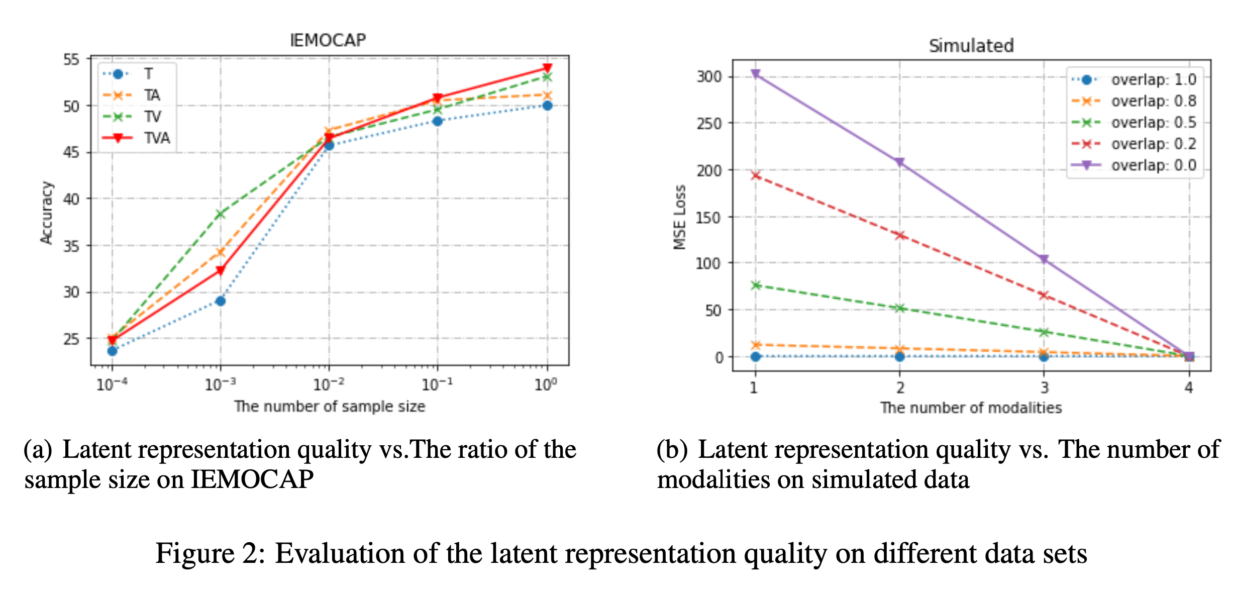
Number of Modalities

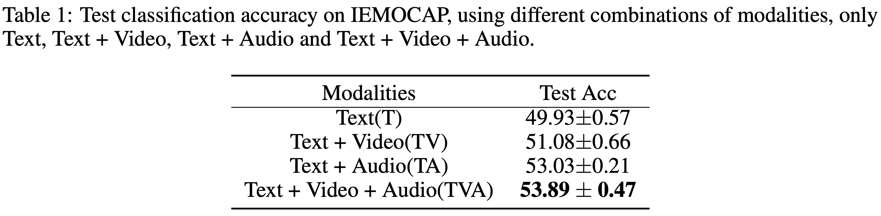
Modal이 늘어날 수록 정확도가 상승하는 것을 볼 수 있다.

Number of Samples

위에서 sample의 수가 클 때 multi-modal이 좋다고 했다. 따라서 이를 살펴보자.

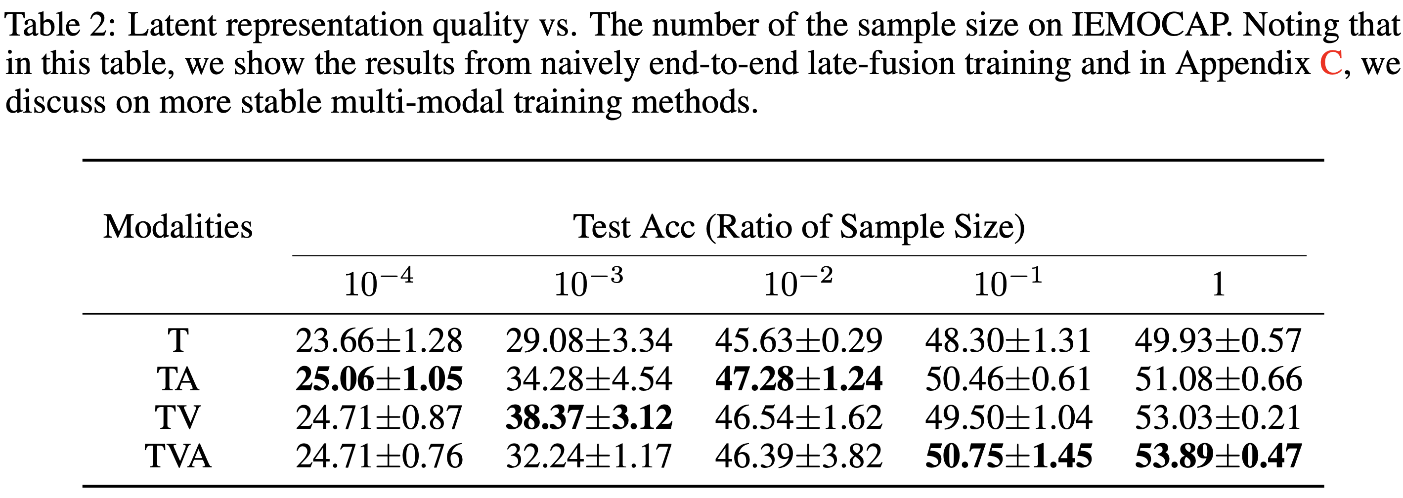
여기서 볼 수 있듯, sample의 수가 줄어들면 madality의 수가 적을 때 성능이 좋은 경우가 있다.

Quality of Latent Spaces

multi-modal은 latent space quality가 좋다고 했다. 이를 확인해보자.

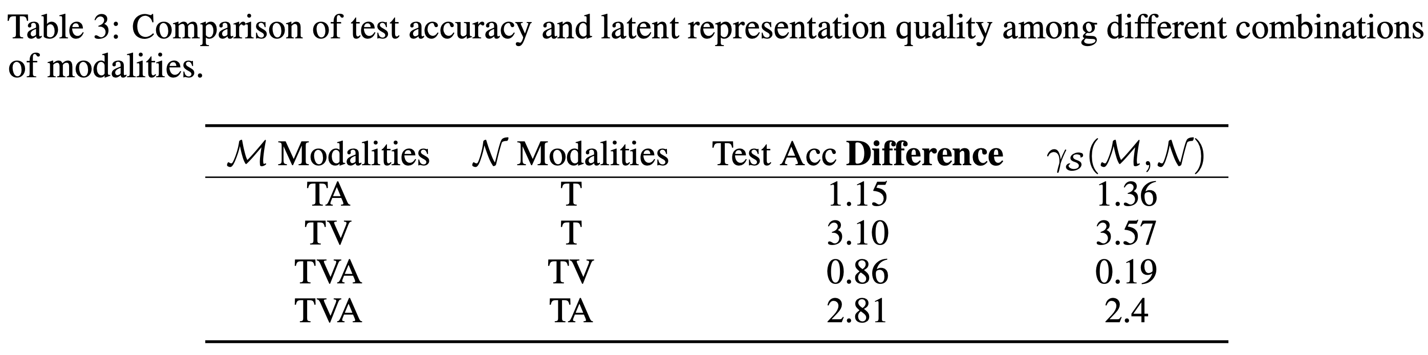
Sample의 수와 modal의 수로 비교해도 같은 결과를 낸다.

Synthetic Data

실제 데이터에서 sample의 수가 많을 때 multi-modal이 좋다는 것을 확인했다. 인공데이터는 어떨까?

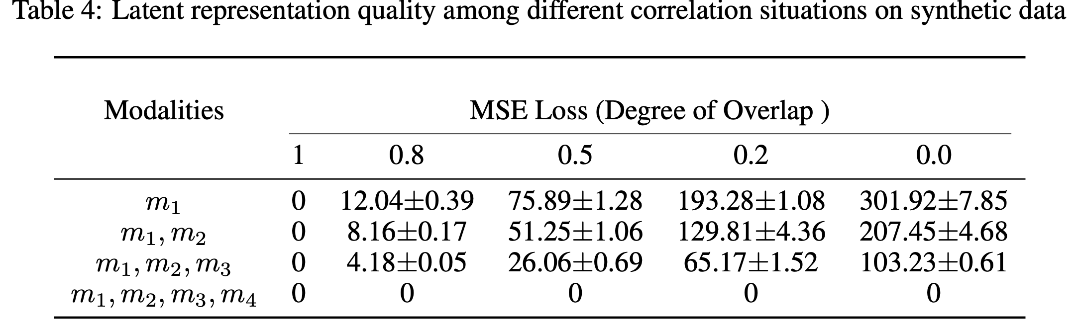
저자가 만든 인공데이터도 같은 모습을 보였다.